
m6AConquer: Methodological Details
Ⅰ. Introduction
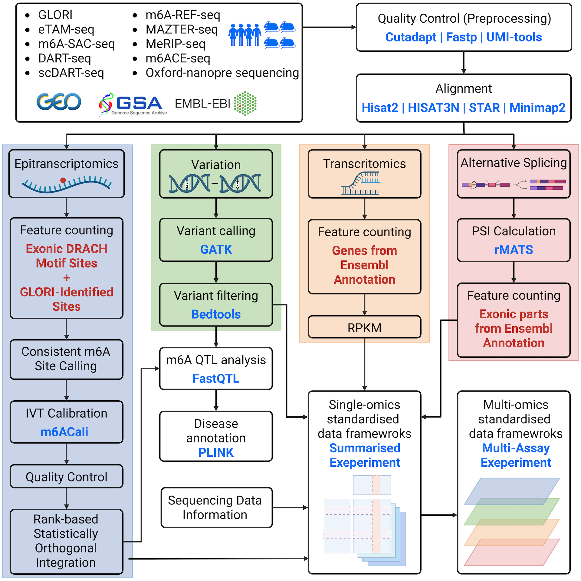
The m6AConquer database offers curated quantitative m6A profiling sequencing data sets. This page provides a brief overview of the processing workflows (Figure 1) utilized to convert raw reads into the data available in this database.
Ⅱ. Data Processing
1. Data gathering
m6AConquer summarises sequencing datasets from 10 different m6A profiling techniques. Both wild type and perturbation samples are included in the database. The perturbation types mainly include the manipulation of m6A-related genes, such as the over-expression of FTO and the knockout of Mettl3. IVT control samples are also included for quantification calibration.
All the sequencing datasets are downloaded from three central database (GEO, GSA, and EMBL-EBI).
2. Quality Control
FastQ read files for NGS techniques are retrieved and downloaded accordingly. Most reads undergo initial trimming using tools like Cutadapt, Trim Galore, and Flexbar to eliminate adaptors and low-quality reads. Some reads are deduplicated through Samtools, Fastx Collapser, and UMI-tools to remove PCR duplications. Fastp is used for both trimming and deduplication.
As for Oxford Nanopore sequencing data, the raw Fast5 files are obtained from the Singapore Nanopore-Expression Project. Quality control is conducted during the basecalling process with Guppy.
The table below summarize the software and tools used in data cleaning and read mapping:
| Techniques | Data cleaning | Read mapping |
|---|---|---|
| DART-seq | Fastp v.0.23.4 | HISAT-3N v.2.2.1-3n-0.0.3 (C → T) |
| eTAM-seq | Cutadapt v.2.9, UMI-tools v.1.1.4 | HISAT-3N v.2.2.1-3n-0.0.3 (A → G) |
| GLORI | Trim Galore v.0.6.6, Fastp v.0.23.4 | STAR v.2.7.11a, bowtie v.1.3.1 |
| m6A-REF-seq | Cutadapt v.2.9 | HISAT2 v.2.1.0 |
| m6A-SAC-seq | Cutadapt v.2.9, Fastx_collapser v.0.0.13 | STAR v.2.7.11a |
| m6ACE | Fastp v.0.23.4 | STAR v.2.7.11a |
| MAZTER-seq | Trim Galore v.0.6.6 | STAR v.2.7.11a |
| MeRIP-seq | Trim Galore v.0.6.6 | HISAT2 v.2.1.0 |
| Oxford-nanopore | Guppy v.3.1.5 (Basecalling) | Minimap2 v.2.17 |
| scDART-seq | Flexbar | STAR v.2.7.11a |
3. Alignment
For NGS sequencing data, 4 aligners (STAR, Bowtie, HISAT2, and HISAT-3N) are utilized for different techniques based on their original pipelines. Bowtie is employed explicitly for transcriptome alignment, while the other three aligners are utilized for genome alignment. The genome index of HISAT2 can be obtained from the provided link: https://genome-idx.s3.amazonaws.com/hisat/grch38_genome.tar.gz. Meanwhile, the genome indexes for STAR and HISAT-3N are constructed as per the specific requirements. All sequencing reads are aligned to the GRCh38 or hg38 human genome, and various versions of gene annotation from RefSeq, Genecode, and Ensemble are employed under their original pipelines. The codes for index building can be accessed on GitHub.
In the context of Oxford Nanopore sequencing data, the aligner minimap2 is utilized for transcriptome alignment. The Ensemble transcript reference of GRCh38 is indexed using the default parameters of minimap2.
4. Feature counting
The m6AConquer database summarizes quantitative m6A profiling results in the form of SummarizedExperiment (SE) objects. These SE objects summarize the total and m6A read coverages at a consistent range of genomic locations and gene expression levels. The consistent genomic locations consist of 2,526,220 (human)/2,666,051 (mouse) adenosines (A) at the center of exonic DRACH motifs and 262,485 (human)/240,480 (mouse) GLORI m6A sites discovered at non-DRACH locations reported in the supplementary data of GLORI. The m6AConquer database also includes gene expression matrices in SE objects on 58,560 (human) / 55,401 (mouse) genes (Transctipt-Omics).
5. Omics data frameworks
The SummarizedExperiment objects consist of four primary components: row ranges, column data, assays matrices, and metadata.
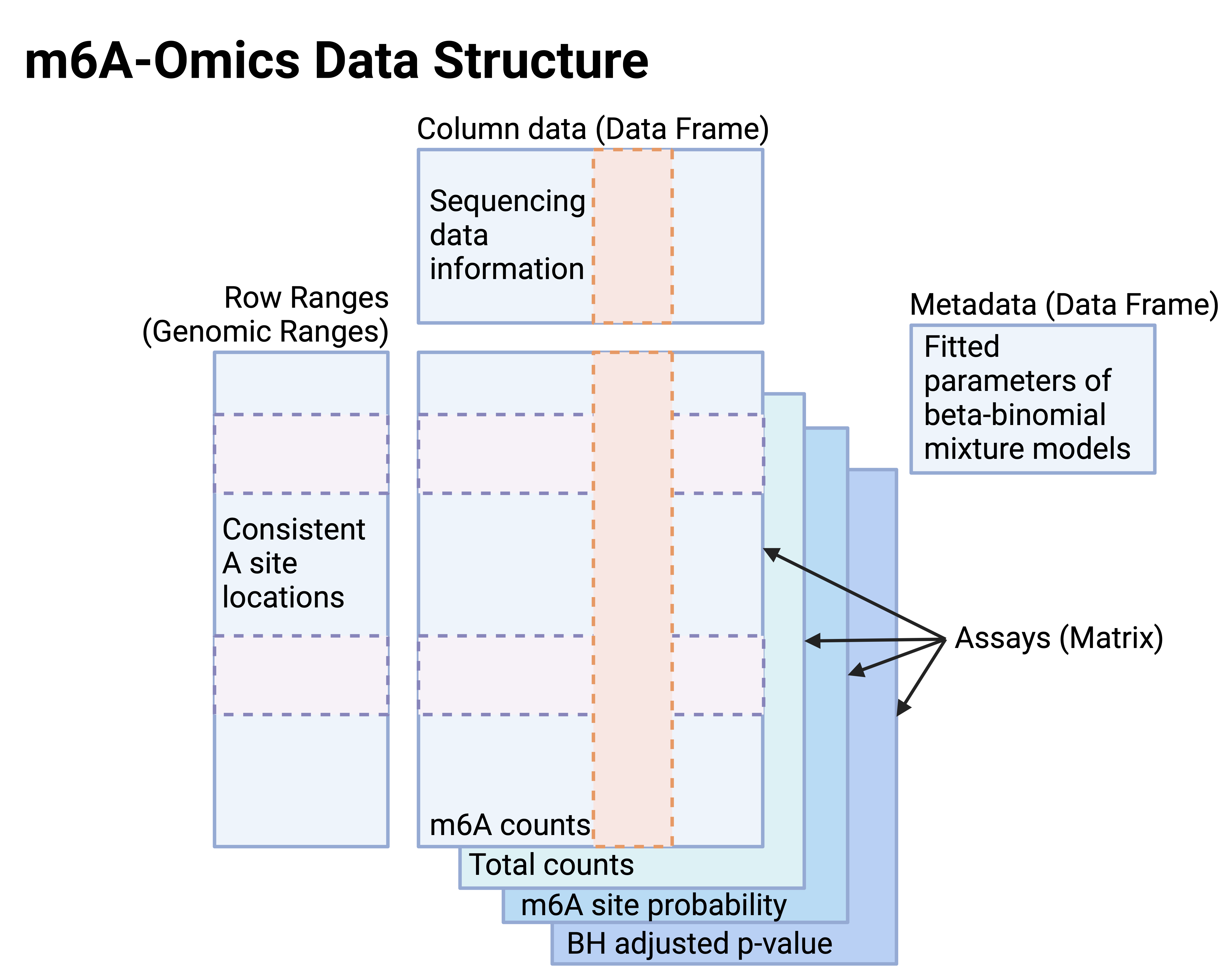
In SE objects for m6A-omics (Figure 2),
- Assays: The matrices for m6A counts and total read coverages at this candidate A sites, m6A site probabilities, and the Benjamini–Hochberg method corrected p-values (FDR).
- Row ranges: Genomic ranges of consistent A locations.
- Column data: Sequencing data information provided by the data generators in the public repositories.
- Metadata: Fitted parameters of m6A site calling and orthogonal reproducible site locations.
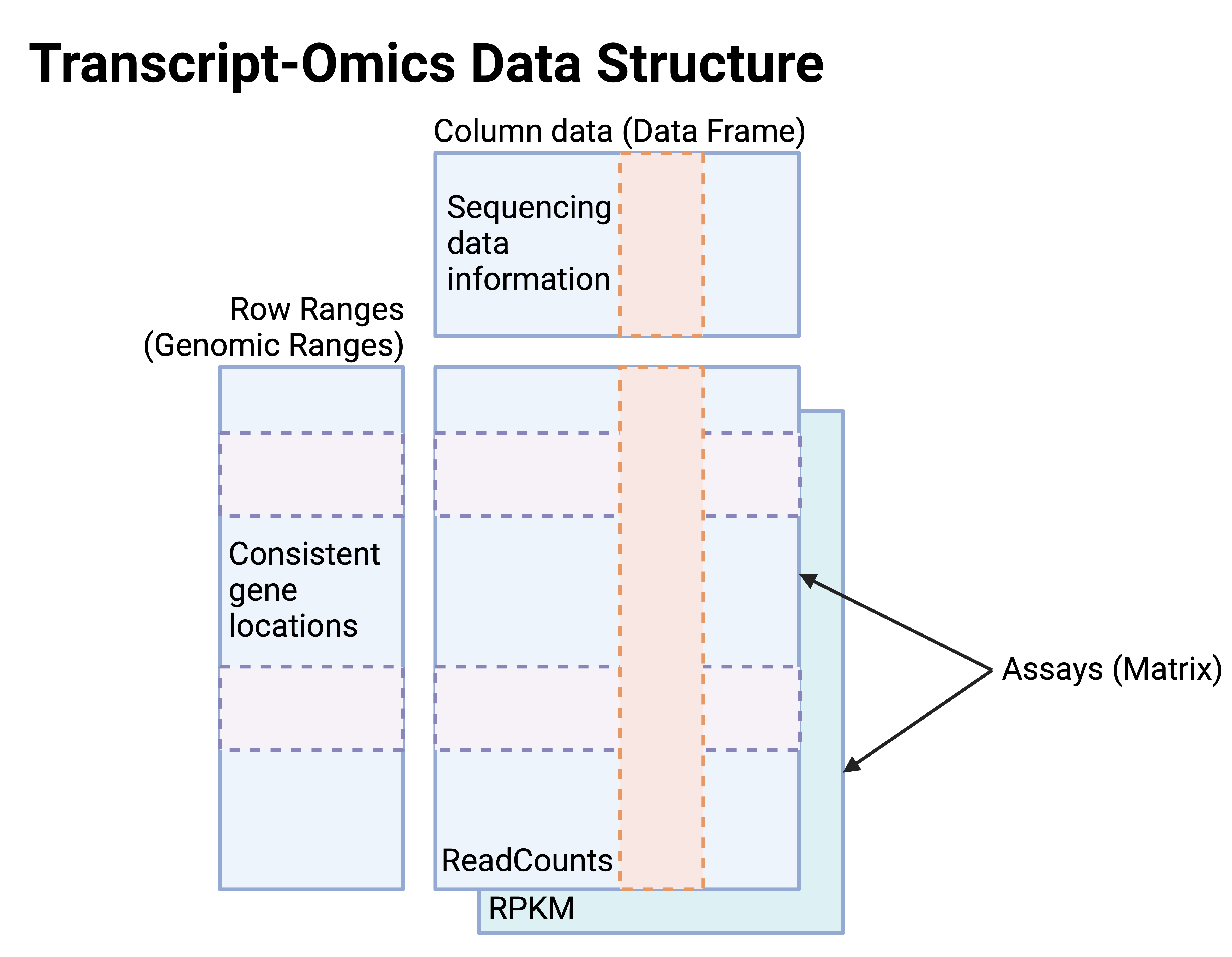
In SE objects for transcript-omics (Figure 3),
- Assays: The matrices for read counts and RPKM at consistent gene features.
- Row ranges: Genomic ranges of gene features.
- Column data: Sequencing data information provided by the data generators in the public repositories, identical to m6A-Omics SE.
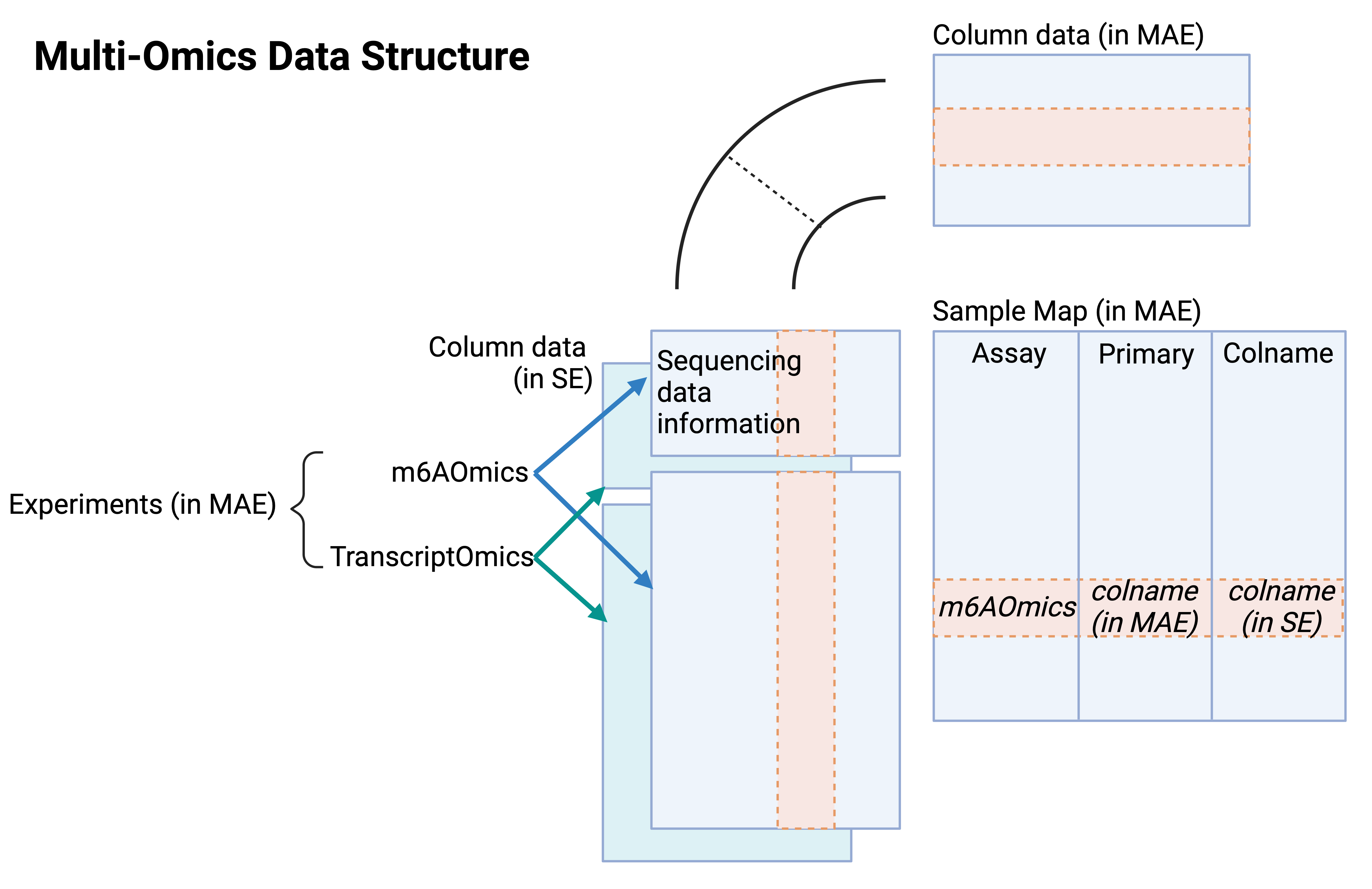
Apart from single-omics data in SE format, multi-omics data in the form of MultiAssayExperiment (MAE) for each profiling technique are also provided. The MAE files are the integration of m6A-Omics and Transcrit-Omics SE objects. The MAE contains distinct components such as experiments, sample maps, and column data for MAE.
In MAE objects for multi-omits (Figure 4),
- Experiments: m6A-Omics and Transcrit-Omics SE objects
- Column data in MAE: The union of column data in all experiment SEs.
- Sample Map: The map relating the column data in experiments to the column data in MAE.
All three types of files can all be downloaded from the Download page.
5. Site calling
m6AConquer consistently used two ways to call m6A sites, the binomial method and the beta-binomial mixture method, on all quantification data to identify m6A sites in various samples. For binomial method, we modeled the observed m6A read counts ()as binomial random variables, where the total read coverage () represented the number of trials. The expected background modification probability () was empirically estimated as the global m6A rate across all positions, calculated as the sum of all m6A reads divided by the sum of all aligned reads:
At each position, a one-sided statistical test was performed under the null hypothesis that the observed m6A count could be explained by the background modification rate. The resulting p-value was computed as the probability of observing at least the measured m6A reads given the site-specific coverage and the global modification probability, following multiple hypothesis correction using Benjamini-Hochberg false discovery rate (FDR) correction.
In addition, we also used a two-component beta-binomial mixture (BBmix) method as an alternative consistent site calling method. The observed m6A read counts () at each site were modeled as a mixture of two beta-binomial distributions representing foreground (methylated) and background (unmethylated) components.
where is the total read coverage, denotes the mixing proportion of methylated sites, and represents the beta-binomial distribution parameterized by mean methylation probabilities ( for background, for foreground) and dispersion parameters (, ). Site-specific posterior methylation probabilities were computed to enable cross-platform comparability:
These probabilities provide normalized methylation confidence scores for downstream integrative analysis.
6. IVT calibration
In the m6AConquer, we have incorporated in vitro transcription (IVT) control samples from GLORI, eTAM-seq, and MeRIP-seq datasets. The IVT control sequencing data from GLORI and eTAM-seq employ the site calling method to identify m6A sites separately. Sites with a false discovery rate (FDR) below 0.05 are considered false positive m6A sites for the respective GLORI or eTAM-seq datasets. In the case of IVT control sequencing data from MeRIP-seq, m6ACali is used to identify false positive m6A sites. For other sequencing data within these three datasets, the m6A counts and total counts at their identified false positive m6A sites are set to 0.
III. Reproducibility-based Orthogonal Integration: IDR analysis
Quantifying reproducibility
To identify reliable modification sites and investigate differences between techniques, m6AConquer implements Irreproducible Discovery Rate (IDR) analysis (Figure 5), a method commonly used in CHIP-seq data to identify consistent peaks in replicates. In our implementation, we evaluate the consistency of identified sites between different techniques, particularly those employing orthogonal mechanisms to quantify m6A abundances.
The underlying assumption of this integration is that the m6A ratios of reproducibility sites should rank higher and more consistently in each pair of techniques. The integration procedure converts paired omics signals from two samples into ranks, which are then modeled them using a two-component bivariate Gaussian copula mixture method. Reproducible m6A sites are identified by positive correlation and consistently high ranks between replicates, while irreproducible m6A sites lack correlation and show inconsistent ranks. Specifically, the IDR value is defined by the posterior probability (responsibility) of the irreproducible component:
where and , denotes the proportion of the reproducible site component, and , , and denote the parameters for the positively correlated bivariate Gaussian distribution. Variables and are continuous signals (m6A ratios by default) measured by two types of m6A profiling techniques respectively at site . and ,are their empirical marginal CDFs used to compute ranks. is a transformation applied in Gaussian copula modeling.
By setting a threshold for the IDR value, the irreproducible discoveries can be controlled. In m6AConquer, this threshold is set to 0.05, which means the overlapped sites with posterior probabilities of belonging to the irreproducible component of less than 5% are considered reproducible.
Technical orthogonal integration
The integration process is conducted between orthogonal technique pairs. Here, ten m6A quantitative profiling techniques are classified into 4 groups based on their sequencing principles:
- Chemical-assisted: Uses specific chemicals to deaminate normal A sites but keep m6A modification sites intact
- Enzyme-assisted: Uses enzymes to capture or cleave at m6A modification sites
- Antibody-assisted: Uses the antibody-immunoprecipitation approach to capture RNA fragments with m6A modifications
- Direct RNA sequencing: Deciphers the m6A modification information by detecting distinct current shift patterns compared to their unmodified counterparts.
Technqiues in different strategy groups are considered orthogonal technique pairs. One exception can be the techniques in antibody-assisted and direct RNA sequencing strategy groups. They are not considered orthogonal because the computational detection method in direct RNA sequencing techniques incorporates m6ACE-seq sequencing results as its training labels. m6ACE-seq is classified in the antibody-assisted strategy group.
In each orthogonal technique pair, overall and condition-specific sample integration methods can be employed. The overall integration method is the sum of m6A counts and total counts at each site from all samples within each technique. As for the condition-specific integration method, summation takes place on samples with common cell lines or tissues.
The reproducibility-based integration results are presented in Genomic Ranges and CSV format in the m6AConquer database. For each orthogonal technique pair, the results contain the genomic locations and IDR values of all reproducible sites, in addition to their m6A methylation ratios, posterior probabilities, and Benjamini-Hochberg (BH) corrected p-values in each technique. Furthermore, a merged Genomic Range and CSV files are provided, containing the union of reproducible sites identified in all orthogonal technique pairs, along with the names and numbers of supported orthogonal technique pairs. Users can access and download these results from the Download page.
IV. Codes
The codes for processing sequencing data is available on GitHub.
The m6A site calling is implemented through OmixM6A R package, which is also available on GitHub.
V. References
Morgan M, Obenchain V, Hester J, Pagès H (2024). SummarizedExperiment: SummarizedExperiment container. R package version 1.34.0, https://bioconductor.org/packages/SummarizedExperiment.
Ramos M, Schiffer L, Re A, Azhar R, Basunia A, Rodriguez Cabrera C, Chan T, Chapman P, Davis S, Gomez-Cabrero D, Culhane A, Haibe-Kains B, Hansen K, Kodali H, Louis M, Mer A, Reister M, Morgan M, Carey V, Waldron L (2017). “Software For The Integration Of Multi-Omics Experiments In Bioconductor.” Cancer Research, 77(21), e39-42. doi:10.1158/0008-5472.CAN-17-0344, https://cancerres.aacrjournals.org/content/77/21/e39.
Qunhua Li. James B. Brown. Haiyan Huang. Peter J. Bickel. "Measuring reproducibility of high-throughput experiments." Ann. Appl. Stat. 5 (3) 1752 - 1779, September 2011. https://doi.org/10.1214/11-AOAS466
Konstantin Krismer, Yuchun Guo, David K Gifford, IDR2D identifies reproducible genomic interactions, Nucleic Acids Research, Volume 48, Issue 6, 06 April 2020, Page e31, https://doi.org/10.1093/nar/gkaa030